This function uses SEMace to find
significant causal effects between source-sink pairs and
SEMpath to fit them and test their edge
perturbation.
Usage
pathFinder(
  graph,
  data,
  group = NULL,
  ace = NULL,
  path = "directed",
  method = "BH",
  alpha = 0.05,
  ...
)
Arguments
- graph
Input network as an igraph object.
- data
A matrix or data.frame. Rows correspond to subjects, and columns to graph nodes (variables).
- group
group A binary vector. This vector must be as long as the number of subjects. Each vector element must be 1 for cases and 0 for control subjects. Group specification enables edge perturbation testing. By default,
group = NULL.- ace
A data.frame generated by
SEMace. If NULL,SEMacewill be automatically run.- path
If
path = "directed", all directed paths between the two nodes will be included in the fitted model. Ifpath = "shortest", only shortest paths will be considered.- method
Multiple testing correction method. One of the values available in
p.adjust. By default,method = "BH"(i.e., FDR multiple test correction).- alpha
Significance level for ACE selection (by default,
alpha = 0.05).- ...
Currently ignored.
Value
A list of 3 objects:
"paths", list of paths as igraph objects;
"fit", fitting results for each path as a lavaan object;
"dfp", a data.frame containing SEM global fitting statistics.
Author
Fernando Palluzzi fernando.palluzzi@gmail.com
Examples
# \donttest{
# Find and evaluate significantly perturbed paths

# Nonparanormal(npn) transformation
als.npn <- transformData(alsData$exprs)$data
#> Conducting the nonparanormal transformation via shrunkun ECDF...done.

adjData <- SEMbap(alsData$graph, als.npn)$data
#> Bow-free covariances search. Use method: cggm ...
#> Number of bow-free covariances / df : 220 / 420
#> Max parent set(S) / Sparsity idx(s) : 10 / 4
#> Number of clusters / number of nodes: 2 / 31
#>

paths <- pathFinder(alsData$graph, adjData,
                    group = alsData$group,
                    ace = NULL)
#>
#>  Frequency distribution of path length from X to Y :
#>  1  2  3  4  5
#> 45 21 16 12  6
#>
#>
 ACE= 1 of 100
 ACE= 2 of 100
 ACE= 3 of 100
 ACE= 4 of 100
 ACE= 5 of 100
 ACE= 6 of 100
 ACE= 7 of 100
 ACE= 8 of 100
 ACE= 9 of 100
 ACE= 10 of 100
 ACE= 11 of 100
 ACE= 12 of 100
 ACE= 13 of 100
 ACE= 14 of 100
 ACE= 15 of 100
 ACE= 16 of 100
 ACE= 17 of 100
 ACE= 18 of 100
 ACE= 19 of 100
 ACE= 20 of 100
 ACE= 21 of 100
 ACE= 22 of 100
 ACE= 23 of 100
 ACE= 24 of 100
 ACE= 25 of 100
 ACE= 26 of 100
 ACE= 27 of 100
 ACE= 28 of 100
 ACE= 29 of 100
 ACE= 30 of 100
 ACE= 31 of 100
 ACE= 32 of 100
 ACE= 33 of 100
 ACE= 34 of 100
 ACE= 35 of 100
 ACE= 36 of 100
 ACE= 37 of 100
 ACE= 38 of 100
 ACE= 39 of 100
 ACE= 40 of 100
 ACE= 41 of 100
 ACE= 42 of 100
 ACE= 43 of 100
 ACE= 44 of 100
 ACE= 45 of 100
 ACE= 46 of 100
 ACE= 47 of 100
 ACE= 48 of 100
 ACE= 49 of 100
 ACE= 50 of 100
 ACE= 51 of 100
 ACE= 52 of 100
 ACE= 53 of 100
 ACE= 54 of 100
 ACE= 55 of 100
 ACE= 56 of 100
 ACE= 57 of 100
 ACE= 58 of 100
 ACE= 59 of 100
 ACE= 60 of 100
 ACE= 61 of 100
 ACE= 62 of 100
 ACE= 63 of 100
 ACE= 64 of 100
 ACE= 65 of 100
 ACE= 66 of 100
 ACE= 67 of 100
 ACE= 68 of 100
 ACE= 69 of 100
 ACE= 70 of 100
 ACE= 71 of 100
 ACE= 72 of 100
 ACE= 73 of 100
 ACE= 74 of 100
 ACE= 75 of 100
 ACE= 76 of 100
 ACE= 77 of 100
 ACE= 78 of 100
 ACE= 79 of 100
 ACE= 80 of 100
 ACE= 81 of 100
 ACE= 82 of 100
 ACE= 83 of 100
 ACE= 84 of 100
 ACE= 85 of 100
 ACE= 86 of 100
 ACE= 87 of 100
 ACE= 88 of 100
 ACE= 89 of 100
 ACE= 90 of 100
 ACE= 91 of 100
 ACE= 92 of 100
 ACE= 93 of 100
 ACE= 94 of 100
 ACE= 95 of 100
 ACE= 96 of 100
 ACE= 97 of 100
 ACE= 98 of 100
 ACE= 99 of 100
 ACE= 100 of 100
#>
 ACE= 1 of 3
 ACE= 2 of 3
 ACE= 3 of 3
#> Found 2 significant ACEs with > 2 nodes
#>

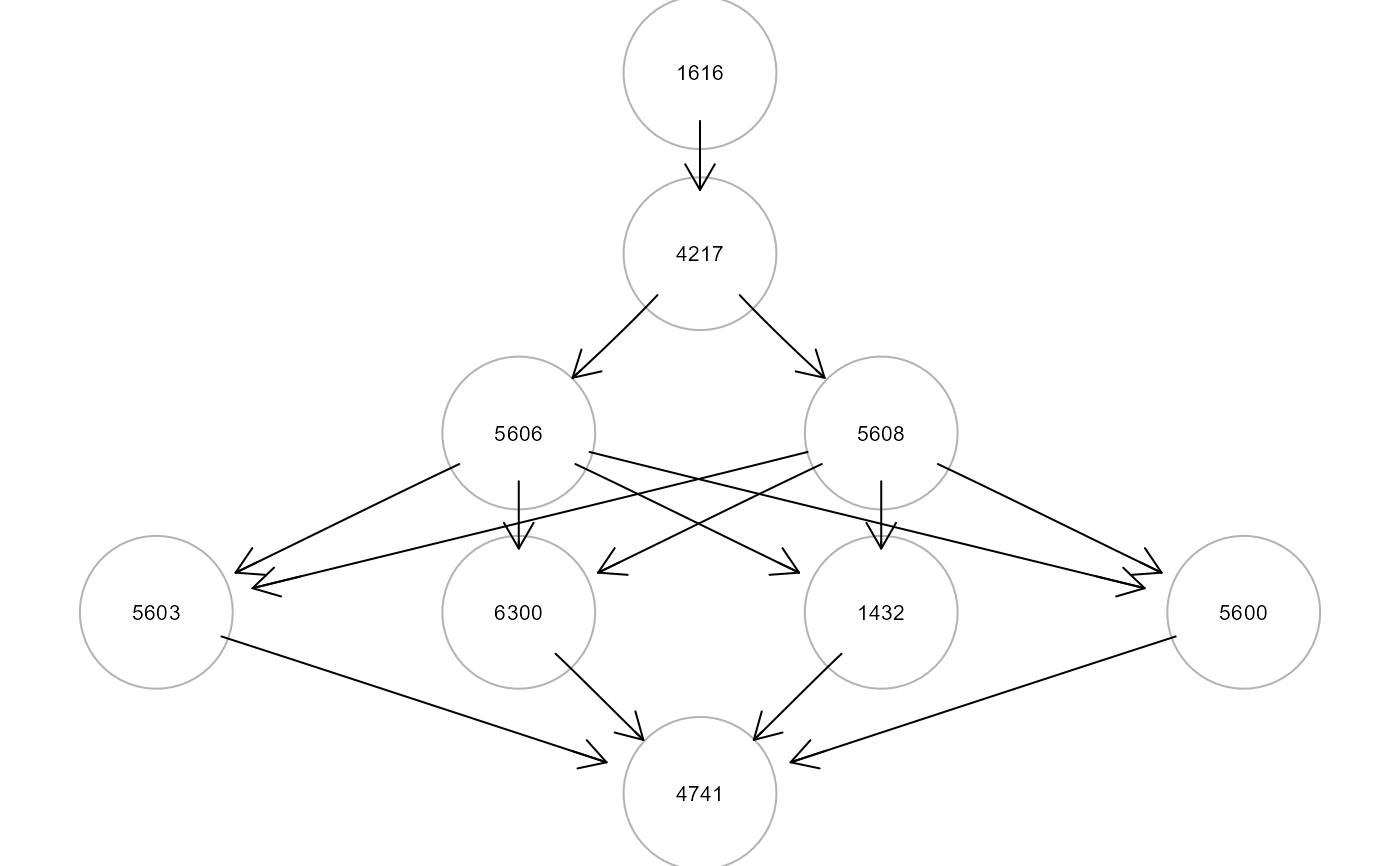
print(paths$dfp)
#>   pathId sink op source n.nodes n.edges dev_df  srmr V.pv.act V.pv.inh
#> 1 P16168 4741 <-   1616       9      15  2.250 0.065 0.000000 0.035968
#> 2  P5962  842 <-    596       3       2  0.369 0.015 0.242861 0.611600
head(parameterEstimates(paths$fit[[1]]))
#>    lhs op   rhs    est    se      z pvalue ci.lower ci.upper
#> 1 1432  ~ group -0.017 0.072 -0.240  0.810   -0.157    0.123
#> 2 1616  ~ group  0.105 0.079  1.329  0.184   -0.050    0.259
#> 3 4217  ~ group  0.062 0.077  0.800  0.424   -0.089    0.212
#> 4 4741  ~ group  0.444 0.073  6.108  0.000    0.302    0.587
#> 5 5600  ~ group -0.296 0.076 -3.911  0.000   -0.445   -0.148
#> 6 5603  ~ group  0.003 0.079  0.032  0.975   -0.153    0.158
gplot(paths$paths[[1]])

# }
# }