Differential Connected Inference (DCI) via a sub-network with
perturbed edges obtained from the output of SEMace,
comparable to the procedure in Jablonski et al (2022), or SEMrun
with two-group and CGGM solver, comparable to the algorithm 2 in Belyaeva et al (2021).
To increase the efficiency of computations for large graphs, users can
select to break the network structure into clusters, and select the
topological clustering method (see clusterGraph).
The function SEMrun is applied iteratively on
each cluster (with size min > 10 and max < 500) to obtain the graph
with the full list of perturbed edges.
Arguments
- graph
Input network as an igraph object.
- data
A matrix or data.frame. Rows correspond to subjects, and columns to graph nodes (variables).
- group
A binary vector. This vector must be as long as the number of subjects. Each vector element must be 1 for cases and 0 for control subjects.
- type
Average Causal Effect (ACE) with two-group, "parents" (back-door) adjustement set, and "direct" effects (
type = "ace", default), or CGGM solver with two-group using a clustering method. Iftype = "tahc", network modules are generated using the tree agglomerative hierarchical clustering method, or non-tree clustering methods from igraph package, i.e.,type = "wtc"(walktrap community structure with short random walks),type ="ebc"(edge betweeness clustering),type = "fgc"(fast greedy method),type = "lbc"(label propagation method),type = "lec"(leading eigenvector method),type = "loc"(multi-level optimization),type = "opc"(optimal community structure),type = "sgc"(spinglass statistical mechanics),type = "none"(no breaking network structure into clusters).- method
Multiple testing correction method. One of the values available in
p.adjust. By default, method is set to "BH" (i.e., FDR multiple test correction).- alpha
Significance level (default = 0.05) for edge set selection.
- ...
Currently ignored.
References
Belyaeva A, Squires C, Uhler C (2021). DCI: learning causal differences between gene regulatory networks. Bioinformatics, 37(18): 3067–3069. <https://doi: 10.1093/bioinformatics/btab167>
Jablonski K, Pirkl M, Ćevid D, Bühlmann P, Beerenwinkel N (2022). Identifying cancer pathway dysregulations using differential causal effects. Bioinformatics, 38(6):1550–1559. <https://doi.org/10.1093/bioinformatics/btab847>
Author
Mario Grassi mario.grassi@unipv.it
Examples
# \dontrun{
#load SEMdata package for ALS data with 17K genes:
devtools::install_github("fernandoPalluzzi/SEMdata")
#> Using GitHub PAT from the git credential store.
#> Downloading GitHub repo fernandoPalluzzi/SEMdata@HEAD
#> ── R CMD build ─────────────────────────────────────────────────────────────────
#> * checking for file 'C:\Users\mario\AppData\Local\Temp\RtmpOAP2bs\remotes4f8c15a9b\fernandoPalluzzi-SEMdata-8e6bb5e/DESCRIPTION' ... OK
#> * preparing 'SEMdata':
#> * checking DESCRIPTION meta-information ... OK
#> * checking for LF line-endings in source and make files and shell scripts
#> * checking for empty or unneeded directories
#> * building 'SEMdata_1.1.1.tar.gz'
#>
#> Installing package into 'C:/Users/mario/AppData/Local/Temp/RtmpmWI6Yf/temp_libpath12244a2e6ec9'
#> (as 'lib' is unspecified)
library(SEMdata)
#>
#> Attaching package: 'SEMdata'
#> The following objects are masked from 'package:SEMgraph':
#>
#> alsData, kegg, kegg.pathways
# Nonparanormal(npn) transformation
data.npn<- transformData(SEMdata::alsData$exprs)$data
#> Conducting the nonparanormal transformation via shrunkun ECDF...done.
dim(data.npn) #160 17695
#> [1] 160 17695
# KEGG interactome (max component)
gU <- properties(kegg)[[1]]
#> Frequency distribution of graph components
#>
#> n.nodes n.graphs
#> 1 5007 1
#>
#> Percent of vertices in the giant component: 100 %
#>
#> is.simple is.dag is.directed is.weighted
#> TRUE FALSE TRUE TRUE
#>
#> which.mutual.FALSE which.mutual.TRUE
#> 41122 3164
#summary(gU)
# Modules with ALS perturbed edges using fast gready clustering
gD<- SEMdci(gU, data.npn, alsData$group, type="fgc")
#> modularity = 0.5948128
#>
#> Community sizes
#> 50 51 52 53 54 44 47 48 49 34 37 41 42 43 46 38
#> 2 2 2 2 2 3 3 3 3 4 4 4 4 4 4 5
#> 45 22 24 31 33 36 29 40 28 30 26 35 19 39 15 23
#> 5 6 6 6 6 6 7 7 9 9 10 10 11 11 12 15
#> 25 9 20 32 21 12 18 27 10 14 17 11 13 8 16 6
#> 16 17 17 19 21 22 24 26 32 35 40 61 67 71 72 134
#> 5 7 2 4 3 1
#> 145 357 364 865 886 1529
#>
#> fit cluster = 1
#> fit cluster = 2
#> fit cluster = 3
#> fit cluster = 4
#> fit cluster = 5
#> fit cluster = 6
#> fit cluster = 7
#> fit cluster = 8
#> fit cluster = 9
#> fit cluster = 10
#> fit cluster = 11
#> fit cluster = 12
#> fit cluster = 13
#> fit cluster = 14
#> fit cluster = 15
#> fit cluster = 16
#> fit cluster = 17
#> fit cluster = 18
#> fit cluster = 19
#> fit cluster = 20
#> fit cluster = 21
#> fit cluster = 23
#> fit cluster = 25
#> fit cluster = 26
#> fit cluster = 27
#> fit cluster = 32
#> fit cluster = 35
#> fit cluster = 39
#> Done.
summary(gD)
#> IGRAPH 77a2c1f DN-- 214 225 --
#> + attr: name (v/c)
gcD<- properties(gD)
#> Frequency distribution of graph components
#>
#> n.nodes n.graphs
#> 1 2 12
#> 2 3 5
#> 3 4 2
#> 4 6 2
#> 5 7 2
#> 6 10 1
#> 7 16 2
#> 8 25 1
#> 9 74 1
#>
#> Percent of vertices in the giant component: 34.6 %
#>
#> is.simple is.dag is.directed is.weighted
#> TRUE TRUE TRUE FALSE
#>
#> which.mutual.FALSE
#> 79
old.par <- par(no.readonly = TRUE)
par(mfrow=c(2,2), mar=rep(2,4))
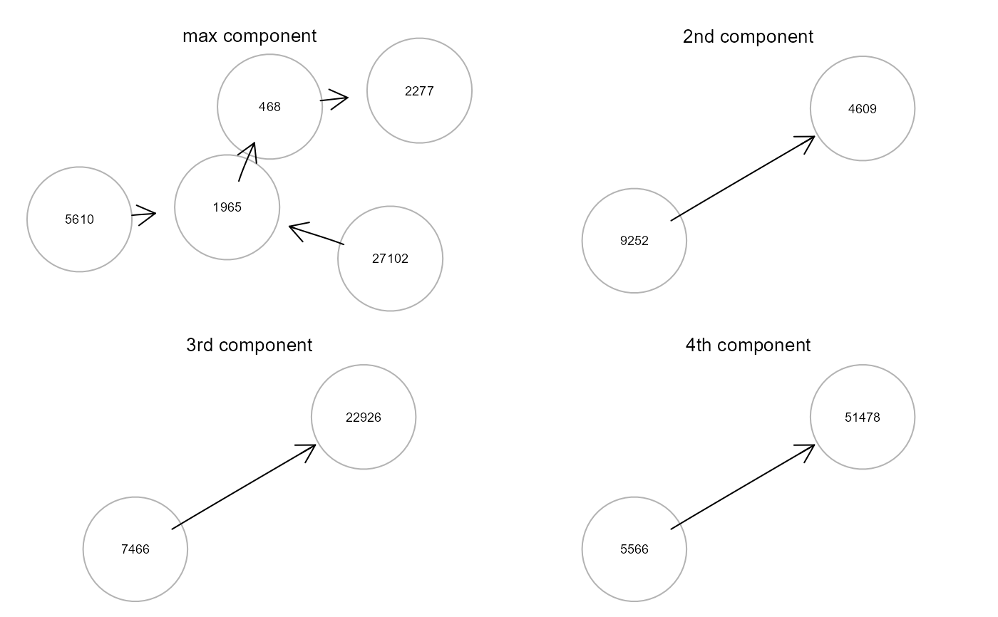
gplot(gcD[[1]], l="fdp", main="max component")
gplot(gcD[[2]], l="fdp", main="2nd component")
gplot(gcD[[3]], l="fdp", main="3rd component")
gplot(gcD[[4]], l="fdp", main="4th component")
 par(old.par)
# }
par(old.par)
# }